Identifying Active and Alternative Promoters from RNA-Seq data with proActiv

Summary

Most human genes have multiple promoters that control the expression of distinct isoforms. The use of these alternative promoters enables the regulation of isoform expression pre-transcriptionally. Alternative promoters have been found to be important in a wide number of cell types and diseases.

proActiv is a method that enables the analysis of promoters from RNA-Seq data. proActiv uses aligned reads as input, and then generates counts and normalized promoter activity estimates for each annotated promoter. These estimates can then be used to identify which promoter is active, which promoter is inactive, and which promoters change their activity across conditions.

Here we present a quick start guide to using proActiv, and a detailed workflow for identifying active promoters and alternative promoters across 2 conditions.

If you use proActiv in your research, please cite:

Demircioğlu, Deniz, et al. “A Pan-cancer Transcriptome Analysis Reveals Pervasive Regulation through Alternative Promoters.” Cell 178.6 (2019): 1465-1477.

Quick Start: Quantifying promoter activity with proActiv
A complete workflow to identify alternative promoter usage
Analysis and visualization of alternative promoter usage
Getting help
Citing proActiv
Session information

Quick Start: Quantifying promoter activity with proActiv

proActiv estimates promoter activity from RNA-Seq data. Promoter activity is defined as the total amount of transcription initiated at each promoter. proActiv takes as input either BAM files or junction files (TopHat2 or STAR), and a promoter annotation object of the relevant genome. An optional argument condition can be supplied, describing the condition corresponding to each input file. Here we demonstrate proActiv with STAR junction files (Human genome GRCh38 Gencode v34) as input. Due to size constraints, analysis is restricted to a subset of chr1 (10,000,000-30,000,000).

library(proActiv)

## List of STAR junction files as input
files <- list.files(system.file('extdata/vignette/junctions', 
                                package = 'proActiv'), full.names = TRUE)
## Vector describing experimental condition
condition <- rep(c('A549','HepG2'), each=3)
## Promoter annotation for human genome GENCODE v34 restricted to a subset of chr1
promoterAnnotation <- promoterAnnotation.gencode.v34.subset

result <- proActiv(files = files, 
                   promoterAnnotation = promoterAnnotation,
                   condition = condition)

result is a summarizedExperiment object which can be accessed as follows:

assays(results) returns raw/normalized promoter counts, absolute/relative promoter activity and gene expression
rowData(results) returns promoter metadata and summarized absolute promoter activity and gene expression by conditions

A complete workflow to identify alternative promoter usage

Here we present a complete step-by-step workflow for analyzing promoter activity with proActiv and for identifying alternative promoter usage across samples from different conditions. We will compare samples from 2 different cell lines (A549 and HepG2) to identify alternative promoters.

Preparing input data

proActiv uses RNA-Seq data to quantify promoter activity. Users have the option of using as input either BAM files, or tab-delimited junction files that are generated when TopHat2 or STAR is used for read alignment.

Below, we demonstrate running proActiv with input STAR junction files. This data is taken from the SGNEx project, and restricted to the chr1:10,000,000-30,000,000 region. The reference genome used for alignment is Gencode v34 (GRCh38). These files can be found in extdata/vignette/junctions:

extdata/vignette/SGNEx_A549_Illumina_replicate1-run1.subset.SJ.out.tab.gz
extdata/vignette/SGNEx_A549_Illumina_replicate3-run1.subset.SJ.out.tab.gz
extdata/vignette/SGNEx_A549_Illumina_replicate5-run1.subset.SJ.out.tab.gz
extdata/vignette/SGNEx_HepG2_Illumina_replicate2-run1.subset.SJ.out.tab.gz
extdata/vignette/SGNEx_HepG2_Illumina_replicate4-run1.subset.SJ.out.tab.gz
extdata/vignette/SGNEx_HepG2_Illumina_replicate5-run1.subset.SJ.out.tab.gz

files <- list.files(system.file('extdata/vignette/junctions', 
                                package = 'proActiv'), full.names = TRUE)

Preparing promoter annotations

In order to quantify promoter activity, proActiv uses a set of promoters based on genome annotations. proActiv allows the creation of a promoter annotation object for any genome from a TxDb object or from a GTF file with the preparePromoterAnnotation function. Users have the option to either pass the file path of the GTF/GFF or TxDb to be used, or use the TxDb object directly as input. proActiv includes pre-calculated promoter annotations for the human genome (GENCODE v34). However, due to size constraints, the annotation is restricted to the chr1:10,000,000-30,000,000 region. Users can build full annotations by downloading GTF files from GENCODE page and following the steps below.

We demonstrate creating the restricted promoter annotation for the Human genome (GENCODE v34) with both GTF and TxDb:

## From GTF file path
gtf.file <- system.file('extdata/vignette/annotation/gencode.v34.annotation.subset.gtf.gz', 
                        package = 'proActiv')
promoterAnnotation.gencode.v34.subset <- preparePromoterAnnotation(file = gtf.file,
                                                                   species = 'Homo_sapiens')
## From TxDb object
txdb.file <- system.file('extdata/vignette/annotation/gencode.v34.annotation.subset.sqlite', 
                         package = 'proActiv')
txdb <- loadDb(txdb.file)
promoterAnnotation.gencode.v34.subset <- preparePromoterAnnotation(txdb = txdb, 
                                                                   species = 'Homo_sapiens')

The PromoterAnnotation object has 3 slots:

intronRanges : Intron ranges, giving the corresponding transcripts of each intron
promoterIdMapping : An ID mapping between transcripts, promoter IDs and gene IDs
promoterCoordinates : Promoter coordinates (TSS) and internal promoter state, along with the 3’ coordinate of the first exon

When creating promoter annotations for other species, one can call genomeStyles to identify the species argument to be used:

names(GenomeInfoDb::genomeStyles())
#>  [1] "Arabidopsis_thaliana"     "Caenorhabditis_elegans"  
#>  [3] "Canis_familiaris"         "Cyanidioschyzon_merolae" 
#>  [5] "Drosophila_melanogaster"  "Homo_sapiens"            
#>  [7] "Mus_musculus"             "Oryza_sativa"            
#>  [9] "Populus_trichocarpa"      "Rattus_norvegicus"       
#> [11] "Saccharomyces_cerevisiae" "Zea_mays"

Running proActiv

Once promoters in the genome are identified, proActiv estimates promoter activity at each annotated promoter. Here, we load pre-calculated promoter annotation for GENCODE Release 34. We also supply the experimental condition to proActiv. This information allows proActiv to summarize results across conditions.

promoterAnnotation <- promoterAnnotation.gencode.v34.subset

condition <- rep(c('A549', 'HepG2'), each=3)

result <- proActiv(files = files,
                   promoterAnnotation = promoterAnnotation,
                   condition = condition)

result is a SummarizedExperiment object with assays as raw/normalized promoter counts, absolute/relative promoter activity and gene expression:

show(result)
#> class: SummarizedExperiment 
#> dim: 1380 6 
#> metadata(0):
#> assays(5): promoterCounts normalizedPromoterCounts
#>   absolutePromoterActivity relativePromoterActivity geneExpression
#> rownames(1380): 1 2 ... 1379 1380
#> rowData names(14): promoterId geneId ... A549.class HepG2.class
#> colnames(6): SGNEx_A549_Illumina_replicate1.run1.subset.SJ.out
#>   SGNEx_A549_Illumina_replicate3.run1.subset.SJ.out ...
#>   SGNEx_HepG2_Illumina_replicate4.run1.subset.SJ.out
#>   SGNEx_HepG2_Illumina_replicate5.run1.subset.SJ.out
#> colData names(2): sampleName condition

The rowData slot stores a promoter-gene ID mapping and promoter position (5’ to 3’) for each promoter by gene. Mean absolute promoter activity and gene expression for each condition is also summarized here. Promoters are also categorized into three classes. Promoters with activity < 0.25 are classified as inactive, while the most active promoters of each gene are classified as major promoters. Promoters active at lower levels are classified as minor promoters.

promoterId	geneId	seqnames	start	strand	internalPromoter	promoterPosition	txId	A549.mean	A549.gene.mean	HepG2.mean	HepG2.gene.mean	A549.class	HepG2.class
1	ENSG00000000938.13	chr1	27624062	-	TRUE	4	ENST0000….	0.000000	0.00000	0.000000	0.00000	NA	NA
2	ENSG00000000938.13	chr1	27626240	-	FALSE	3	ENST0000….	0.000000	0.00000	0.000000	0.00000	Inactive	Inactive
3	ENSG00000000938.13	chr1	27626569	-	FALSE	2	ENST0000….	0.000000	0.00000	0.000000	0.00000	Inactive	Inactive
4	ENSG00000000938.13	chr1	27635185	-	FALSE	1	ENST0000….	0.000000	0.00000	0.000000	0.00000	Inactive	Inactive
5	ENSG00000001460.18	chr1	24379823	-	TRUE	7	ENST0000….	4.721803	20.91493	4.319706	18.81489	NA	NA
6	ENSG00000001460.18	chr1	24391679	-	TRUE	6	ENST0000….	4.207194	20.91493	3.999170	18.81489	NA	NA

For cleaner downstream analysis, one can remove single-exon transcripts for which promoter activity is not quantified. result can be filtered as such:

## Removes single-exon transcripts / promoters by eliminating promoter counts that are NA 
result <- result[complete.cases(assays(result)$promoterCounts),]

Identifying alternative promoters

To identify alternative promoter usage, proActiv implements a linear model, regressing both absolute promoter activity and relative promoter activity against sample conditions. A change in absolute promoter activity indicates absolute differential usage of the promoter. However, this does not imply alternative usage or a switch in major promoter, as the relative usage of promoters between conditions may still be the same. For this reason, information from relative promoter activity must also be taken into account. Alternative promoter usage is thus characterized by a significant change in absolute and relative promoter activity across conditions.

Candidates for alternative promoter usage can be identified by calling getAlternativePromoters. This function takes in the result object returned by proActiv, and referenceCondition, the reference condition to be compared to all other samples.

alternativePromoters <- getAlternativePromoters(result = result, referenceCondition = "A549")
#> Fitting absolute promoter activity to condition...
#> Fitting relative promoter activity to condition...
show(alternativePromoters)
#> $upReg
#>     promoterId             geneId     padjAbs    padjRel
#> 137        137 ENSG00000076864.19 0.004137450 0.03624923
#> 138        138 ENSG00000076864.19 0.009286492 0.03364840
#> 314        314 ENSG00000117632.23 0.002433754 0.02968373
#> 
#> $downReg
#>     promoterId             geneId     padjAbs   padjRel
#> 141        141 ENSG00000076864.19 0.007574438 0.0336484

Detection of alternative promoters with the following parameters:

minAbs Minimum value for promoter to be active in absolute terms. Defaults to 0.25.
minRel Minimum value for promoter to be active in relative terms. Defaults to 0.05.
maxPval Adjusted p-value threshold for detecting alternative promoters. Defaults to 0.05.
promoterFC Minimum fold change for a promoter in the current condition compared to all other conditions. Promoters must have at least this magnitude of fold change for alternative usage. This parameter can be decreased to relax alternative usage definition. Defaults to 2.0.
geneFC Maximum fold change for gene expression. To identify alternative promoter usage independent of changes in gene expression, limit the gene expression fold change. Promoters must have at most this magnitude of gene expression fold change for alternative usage. This parameter can be increased to relax alternative usage definition. Defaults to 1.5.

Analysis and visualization of alternative promoter usage

Here we offer several visualizations of the data returned by the workflow above.

Alternative Promoter Usage

To visualize genes with alternative promoter usage across conditions, the function boxplotPromoters can be used. This function outputs boxplots of gene expression, absolute and relative promoter activity for a gene of interest. boxplotPromoters takes the following arguments:

result. The summarizedExperiment object returned by proActiv. This must contain a condition vector (i.e., the call to proActiv that returned this result must have had the condition vector supplied).
geneId. A character vector of the gene of interest. This identifier must correspond to the identifier in the promoter annotation.
geneName. A character vector of the gene of interest. The common gene name to be plotted. Optional and defaults to NULL.
filterInternal. A boolean variable that determines if internal promoters should be removed from the plot. Defaults to TRUE.
col. A character vector of colours for plotting. Defaults to NULL, which uses ggplot2 default colours.

Below, we call boxplotPromoters with RAP1GAP:

plots <- boxplotPromoters(result, "ENSG00000076864.19")

# Boxplot of absolute promoter activity
library(gridExtra)
grid.arrange(plots[[1]], plots[[3]], nrow = 1, ncol = 2, widths = c(3, 2))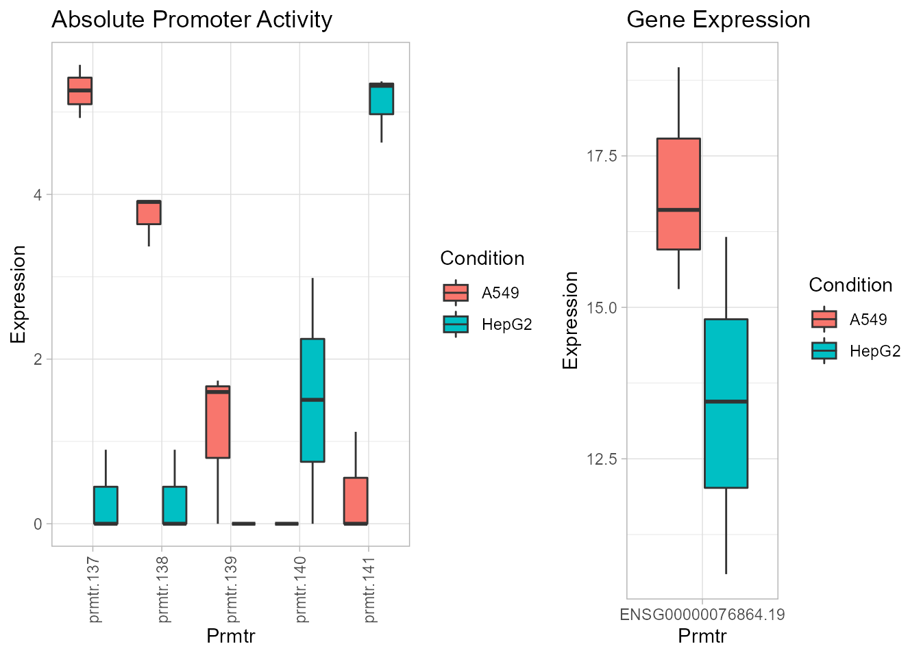

The plots object stores the plot for absolute promoter activity, relative promoter activity and gene expression in the first, second and third slot respectively. The plot generated by boxplotPromoters reflect the alternative usage of promoters 137 and 141 as called by getAlternativePromoters.

Promoter category proportion

Here, we visualize the categorization of annotated promoters in the two cell lines. The proportions between the categories are similar across the two cell lines, with majority of the promoters being inactive.

library(ggplot2)

rdata <- rowData(result)
## Create a long dataframe summarizing cell line and promoter class
pdata1 <- data.frame(cellLine = rep(c('A549', 'HepG2'), each = nrow(rdata)),
                       promoterClass = as.factor(c(rdata$A549.class, rdata$HepG2.class)))

ggplot(na.omit(pdata1)) +
  geom_bar(aes(x = cellLine, fill = promoterClass)) + 
  xlab('Cell Lines') + ylab('Count') +  labs(fill = 'Promoter Category') +
  ggtitle('Categorization of Promoters')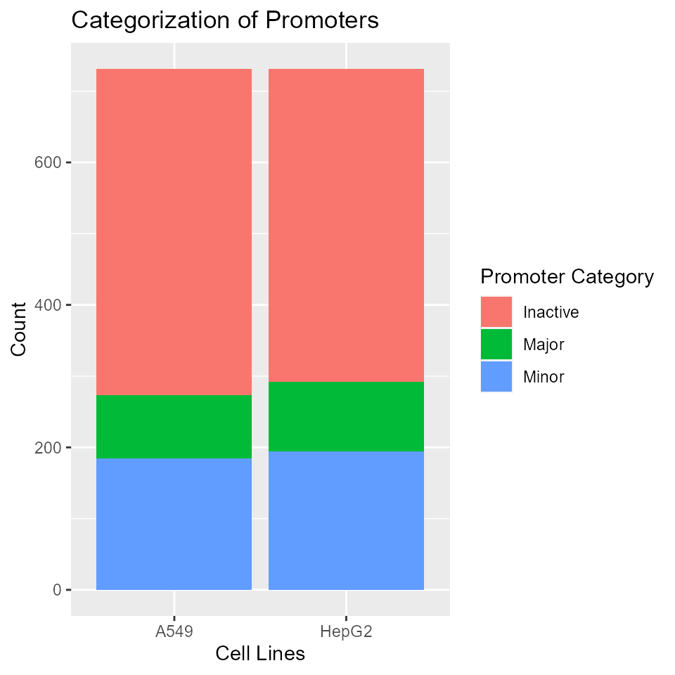

Major/minor promoters by position

Analysis of major:minor promoter proportions against promoter position. The analysis is restricted to multi-promoter genes with at least one active promoter. Below, we generate the plot for cell line HepG2. In general, the major:minor promoter proportion decreases with increasing promoter position.

## Because many genes have many annotated promoters, we collapse promoters 
## from the 5th position and onward into one group for simplicity
pdata2 <- as_tibble(rdata) %>%
  mutate(promoterPosition = ifelse(promoterPosition > 5, 5, promoterPosition)) %>%
  filter(HepG2.class %in% c('Major', 'Minor'))

ggplot(pdata2) +
  geom_bar(aes(x = promoterPosition, fill = as.factor(HepG2.class)), position = 'fill') +
  xlab(expression(Promoter ~ Position ~ "5'" %->% "3'")) + ylab('Percentage') + 
  labs(fill = 'Promoter Category') + ggtitle('Major/Minor Promoter Proportion in HepG2') + 
  scale_y_continuous(breaks = seq(0,1, 0.25), labels = paste0(seq(0,100,25),'%')) +
  scale_x_continuous(breaks = seq(1,5), labels = c('1','2','3','4','>=5'))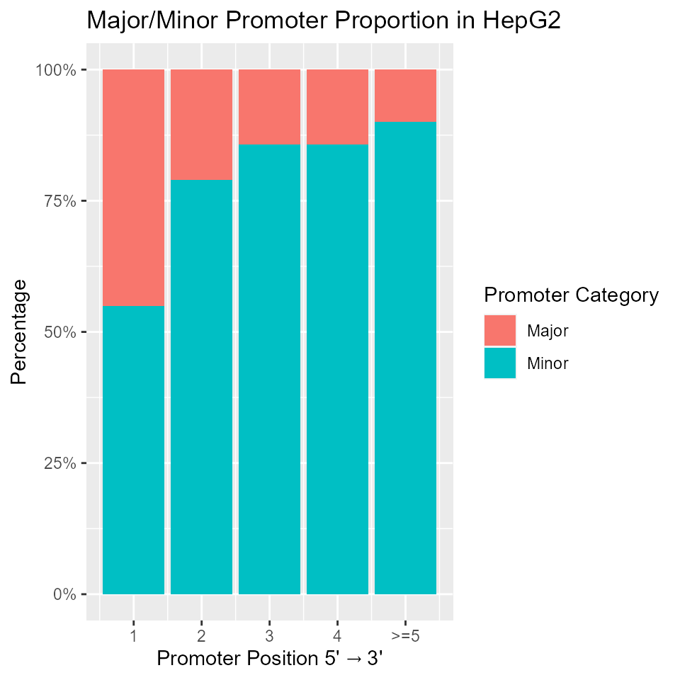

Major promoter activity and gene expression

Comparison of major promoter activity and gene expression, calculated by summing over all promoters. Single promoter genes lie on the diagonal. Multi-promoter genes lie to the right of the diagonal. Below, we generate the plot for cell line HepG2. This plot suggests that a single major promoter does not often fully explain gene expression, with minor promoters also contributing to gene expression.

## Get active major promoters of HepG2
majorPromoter <- as_tibble(rdata) %>% group_by(geneId) %>% 
  mutate(promoterCount = n()) %>% filter(HepG2.class == 'Major') 

pdata3 <- data.frame(proActiv = majorPromoter$HepG2.mean,
                     geneExp = majorPromoter$HepG2.gene.mean,
                     promoterCount = majorPromoter$promoterCount)

ggplot(pdata3, aes(x = geneExp, y = proActiv)) + 
  geom_point(aes(colour = promoterCount), alpha = 0.5) +
  ggtitle('Major Promoter Activity vs. Gene Expression in HepG2') + 
  xlab('Average Gene Expression') + ylab('Average Major Promoter Activity') +
  labs(colour = 'Number of \n Annotated Promoters') +
  geom_abline(slope = 1, intercept = 0, colour = 'red', linetype = 'dashed')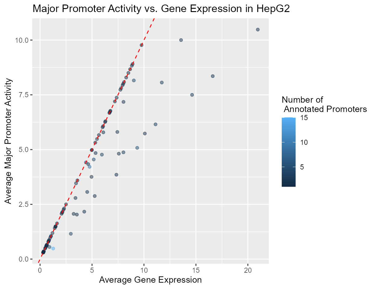

t-SNE

We generate a t-SNE plot with all active promoters. Expectedly, replicates from each cell line cluster together.

library(Rtsne)

## Remove inactive promoters (sparse rows)
data <- assays(result)$absolutePromoterActivity %>% filter(rowSums(.) > 0)
data <- data.frame(t(data))
data$Sample <- as.factor(condition)

set.seed(40) # for reproducibility

tsne.out <- Rtsne(as.matrix(subset(data, select = -c(Sample))), perplexity = 1)
plot(x = tsne.out$Y[,1], y = tsne.out$Y[,2], bg = data$Sample, asp = 1,
     col = 'black', pch = 24, cex = 4,
     main = 't-SNE plot with promoters \n active in at least one sample',
     xlab = 'T-SNE1', ylab = 'T-SNE2',
     xlim = c(-300,300), ylim = c(-300,300))
legend('topright', inset = .02, title = 'Cell Lines',
       unique(condition), pch = c(24,24), pt.bg = 1:length(unique(condition)) , cex = 1.5, bty = 'n')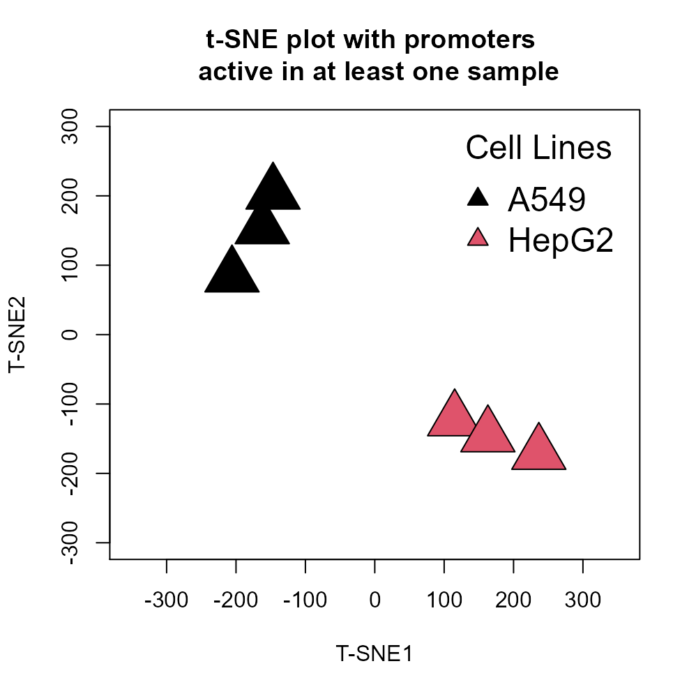

Getting help

Questions and issues can be raised at the Bioconductor support site: https://support.bioconductor.org. Ensure your posts are tagged with proActiv.

Alternatively, issues can be raised at the proActiv Github repository: https://github.com/GoekeLab/proActiv.

Citing proActiv

If you use proActiv, please cite: